hydflood - Vignette

Arnd Weber

2024-10-07

Purpose

hydflood is an R package designed to compute flood extent and duration along the German federal waterways Elbe and Rhine.

Use

Installation

The package hydflood is available from CRAN. To install it run:

install.packages("hydflood")

To install the recent developmental version from Github execute the following commands:

install.packages("devtools")
library(devtools)
devtools::install_github("bafg-bund/hydflood")

Afterwards hydflood can be loaded like every other R package with the following command:

options("hydflood.datadir" = tempdir())
library(hydflood)

Dependencies

The package hydflood is built around the packages terra and hyd1d. hyd1d internally provides gauging data for all gauging stations along the rivers Rhine and Elbe operated by the German Waterway and Shipping Administration and computes 1D water levels. The package terra provides the S4 class SpatRaster and thereby enables the GIS based comparison between extrapolated water levels and elevation data.

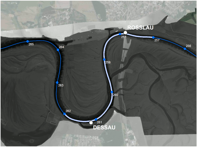
Fig. 1: Digital elevation model of the waterway (DEM-W, in German: Digitales Geländemodell des Wasserlaufs, DGM-W) with 1 m spatial resolution at the River Elbe near Rosslau and Dessau.

hydflood provides download facilities for the digital elevation models of the waterways Rhine and Elbe (DEM, Weber (2020)) with 1 m spatial resolution for chosen extents. If necessary, alternative dem’s can be supplied by users. They just need to overlap with active floodplains of either the Rhine (sf.afr) or the Elbe (sf.afe).

To create a water surface raster, which can be compared to the dem, a simple 1D to 2D conversion is applied to water level data computed along the river axis with the package hyd1d. Therefore so called cross section areas (csa) are needed. They originate from cross sections used for the SOBEK models run for and incorporated into FLYS.

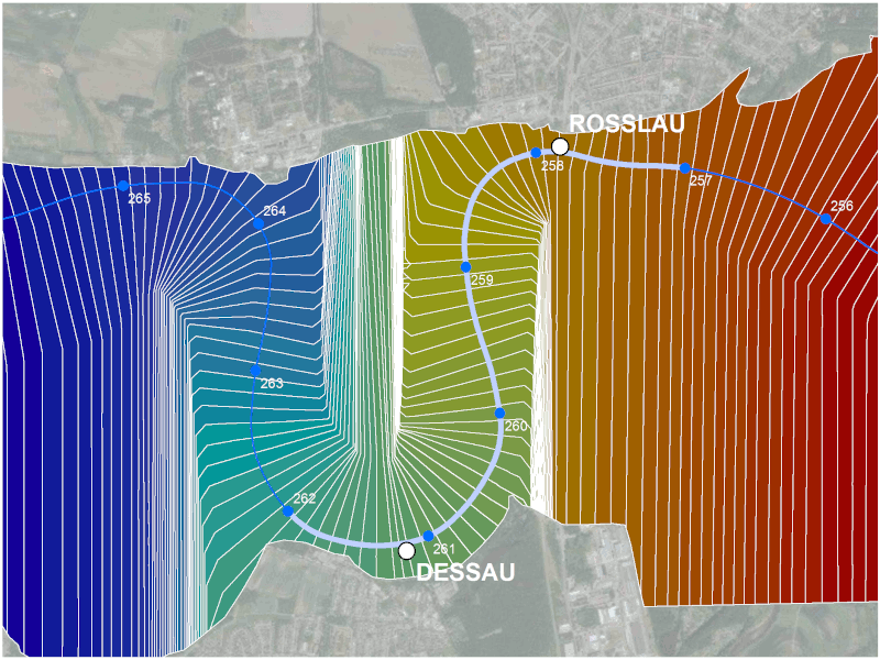
Fig. 2: Cross sections produced to gather input data for SOBEK models used in FLYS at the River Elbe near Rosslau and Dessau.

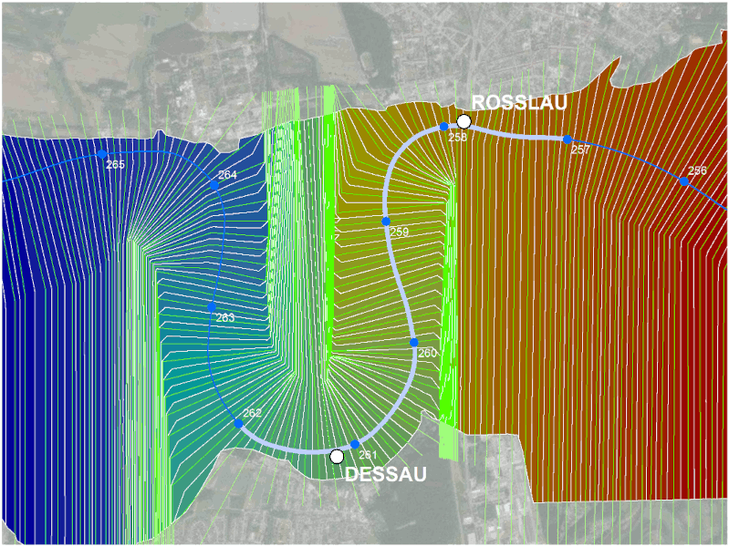
Fig. 3: Cross section areas derived from the cross sections illustrated in Fig. 2 at the River Elbe near Rosslau and Dessau.

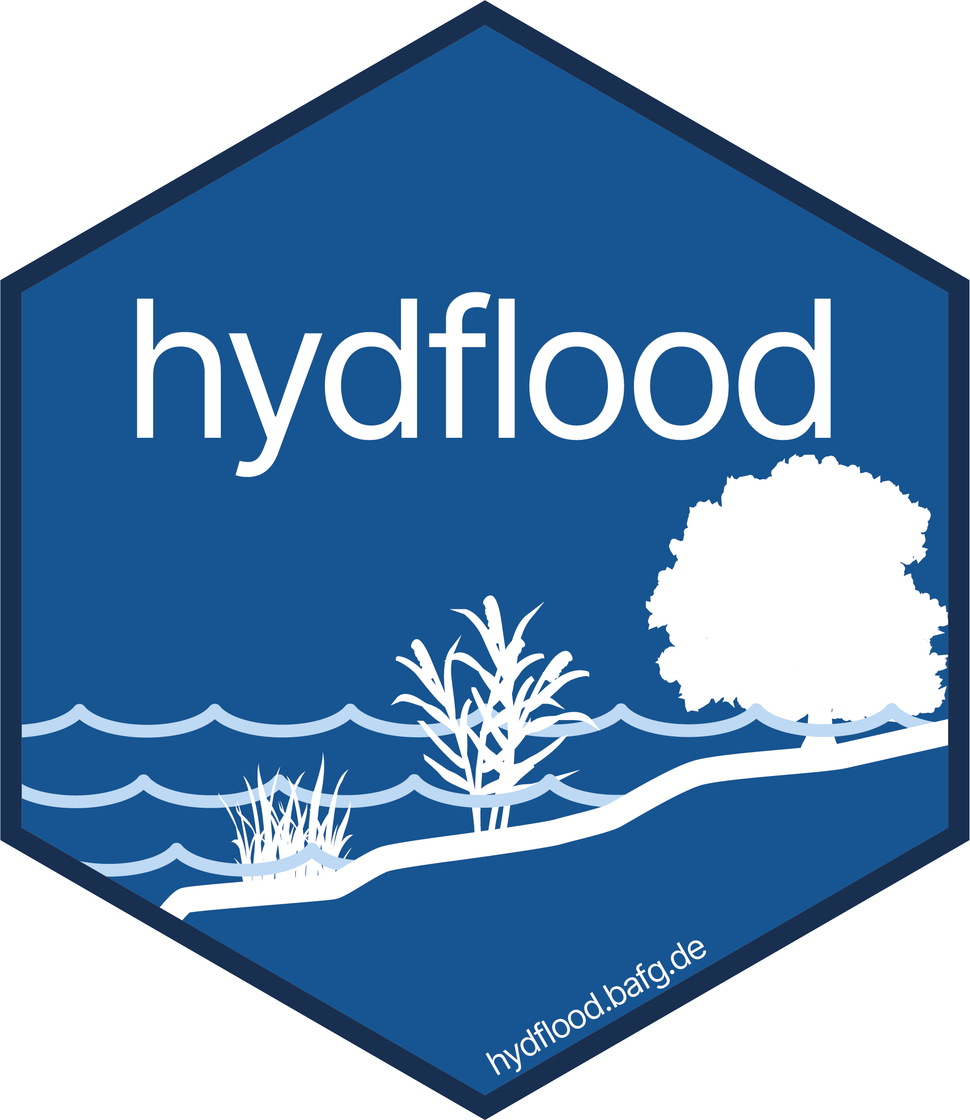
Fig. 4: Cross section areas illustrated in Fig. 3 overlaid by the corresponding cross sections illustrated in Fig. 2 at the River Elbe near Rosslau and Dessau.

These cross sections, one for each individual river station, represent water level isolines perpendicular to the rivers axis. To enable the spatial extrapolation of water level information for each river station, they were converted to cross section areas (csa) which are similar to stairs along the river axis, each step corresponding to a station of the 1D WaterLevelDataFrame computed by the waterLevel function of package hyd1d. To accelerate the computations, while keeping the package size on CRAN small, cross section areas are downloaded once for each river by package internal facilities during their first use.

Computation of flood extents and durations

The actual computation of a flood extent in a selected computational domain for a given time can be split into five steps:

1. Extraction of relevant stations within the computational domain
2. Creation of a WaterLevelDataFrame for the selected river section
3. Computation of the 1D water level using the waterLevel function of package hyd1d
4. Transfer of the 1D water level information from the WaterLevelDataFrame to the cross section areas (csa) through the join field station_int
5. Computation of a binary flood raster fd through the equation fd[csa > dem] = fd[csa > dem] + 1

To compute flood durations these five steps are repeated for every given time step, so that the resulting raster contains counts of how often each individual raster cell was flooded. The possible range of values is between 0 and the number of time steps given.

Usage

To initialize such a SpatRaster several possibilities are implemented in the initializing homonymous function hydSpatRaster. Either you provide a digital elevation model and cross section areas yourself as variables filename_dem and filename_csa or you provide only one of them or you simply provide ext (an object of type SpatExtent) and crs (an object of class CRS). Depending on the supplied coordinate reference system (supplied through either filename_dem, filename_csa or crs) the respective river is selected: For the River Rhine data with ‘ETRS 1989 UTM 32N’ (EPSG 25832) have to be supplied, for the River Elbe ‘ETRS 1989 UTM 32N’ (EPSG 25833). If you can’t provide dem and csa yourself, hydflood provides csa data internally and downloads the official digital elevation models of the German Waterway and Shipping Administration with 1 m spatial resolution. Therefore you definitely need internet access and, due to the data volume of the elevation data, your internet should be fast or you should be patient.

# import the raster data and create a raster stack
x <- hydSpatRaster(filename_dem = "data-raw/raster.dem.tif",
                   filename_csa = "data-raw/raster.csa.tif")

After initialinzig an object of type hydSpatRaster everything else is straight forward. Create a temporal sequence seq:

seq <- seq(as.Date("2016-12-01"), as.Date("2016-12-31"), by = "day")

And supply both of them to the flood3 function, which will do the computation and return an ‘INT4S’ raster with counts of how often the individual cell of the dem was lower than the csa during the temporal sequence. For each time step of the temporal sequence the corresponding 1D WaterLevelDataFrame is computed, joined to csa through the station_int column and compared to the dem so that the possible values of the returned product range between 0 and length(seq):

# compute a flood duration
fd <- flood3(x = x, seq = seq)

# and plot it
plot(fd)

Products

Raster data

Raster data with annual flood durations between 1960 and 2021 for the active floodplains of the River Rhine and the River Elbe have been submitted to and published on pangaea.de (Weber, 2022, 2023).

ShinyApps

flood3daily

The flood3 function is the central function of the package hydflood. With the help of this function daily flood extents are computed for a number of areas along the River Elbe. These products are visualized through a shiny web application available through:

https://shiny.bafg.de/flood3daily/

Fig. 5: Screenshot of the flood3daily-ShinyApp with the modelled flood extent computed for 2016-12-21 at the River Elbe between Rosslau and Dessau, Germany.

flood3wms

The flood3 function is the central function of the package hydflood. With the help of this function annual flood durations between 1990 and 2022 have been computed for the active floodplains of the River Rhine and the River Elbe. These large scale raster products have been visualized as web map services and are available through a shiny web application:

https://shiny.bafg.de/flood3wms/

Fig. 6: Screenshot of the flood3wms-ShinyApp with the annual flood duration of 2016 at the River Elbe between Rosslau and Dessau, Germany.

References

Weber, A. (2020). Digital elevation models of German waterway and navigation authorities - Version 0.1.0. BfG-Bericht, Bundesanstalt für Gewässerkunde, Koblenz, Germany: Bundesanstalt für Gewässerkunde, Koblenz, Germany. https://doi.org/10.5675/BfG-2011

Weber, A. (2022). Flood durations and potential natural vegetation distribution on the floodplains of River Rhine and River Elbe, Germany. data set, PANGAEA. https://doi.org/10.1594/PANGAEA.948042

Weber, A. (2023). Flood durations of the year 2022 on the floodplains of River Rhine and River Elbe, Germany. data set, PANGAEA. https://doi.org/10.1594/PANGAEA.961117

Weber, A., & Hatz, M. (2023). hyd1d: 1d Water Level Interpolation along the Rivers Elbe and Rhine. https://hyd1d.bafg.de/index.html